This page uses
 and
and
 (click images to validate).
You will need a standards-compliant browser to view it properly.
Mozilla 1.x and Opera 6.x are known to work if your default font
contains all mathematical symbols specified by HTML.
Internet Explorer seems to have trouble with some mathematical symbols
even if the font contains them.
Visualization of Natural Deduction as a
Game of Dominoes
©
Matthias S. Benkmann <matthias (a) winterdrache.de>
Abstract
Diagrammatic reasoning systems that allow conducting a proof within a
certain logic have existed for some time, especially as teaching tools.
However, few systems exist that work without any textual formulae.
The domino system presented here is a purely graphical notation for
natural deduction.
A formula is represented as a pattern on a domino tile and a
simple domino game is used as visualisation of a natural
deduction proof.
The game has been implemented as a Java program that acts as an
interactive theorem prover for classical
propositional logic. The program
demonstrates that graphical reasoning systems have some advantages
but also disadvantages. In conjunction with the domino project, a tautology
generator, an interactive theorem prover in text mode and a program that
automatically constructs
a natural deduction proof for a given tautology
have been developed.
1 Introduction
1.1 Reasoning and Diagrams
There are different ways of reasoning. The natural way for
most people is reasoning on the semantic level.
Even mathematicians, although they use precise definitions and
a very formalized way of presentation,
generally conduct proofs using semantic arguments.
Diagrams have always played an important role in this reasoning style.
Another way of reasoning, practiced in its pure form almost
exclusively by logicians, is to work on the syntactic level, using a
formal and abstract language and exact rules
governing the creation and transformation of statements in this language.
The use of diagrams in syntactic reasoning has not found many followers.
One important reason for this is probably that drawing and manipulating
large numbers of diagrams is tedious and inefficient, as is the
typesetting of the results of this process. However, modern computer
technology can help with both issues.
The idea of syntactic reasoning based on diagrams is anything but new.
At the end of the 19th century, when modern mathematics was
still in its infancy, C. S. Peirce suggested a formal deduction
system he
called "Existential Graphs" that is based on diagrams
(for an introduction to this system see [1])
and is as
powerful as first-order logic. Other reasoning systems based on diagrams
have been developed, usually with a more specific area of application,
e.g. a system for reasoning with spider diagrams
(see [2])
.
There are many computer programs that involve diagrammatic reasoning,
usually for teaching purposes. Most of these programs, like for instance
the Hyperproof system
(see [3])
, use diagrams only to support
other reasoning styles. The diagrams employed by these programs and in
fact even the diagrams involved in most reasoning systems that are
syntactic, such as the spider diagrams mentioned above, usually have a
strong semantic element and an intuitive reading.
The program described in this paper is different. Although it does
not implement Peirce's Existential Graphs, it is based on the same idea of
conducting a proof without leaving the diagrammatic level.
Working with such a system is radically different from how proofs are
usually developed. Peirce once wrote:
By diagrammatic reasoning, I mean reasoning which constructs a diagram
according to a precept expressed in general terms, performs experiments
upon this diagram, notes their results, assures itself that similar
experiments
performed upon any diagram constructed according to the same precept would
have same results, and expresses this in general terms. This was a
discovery of no little importance, showing, as it does, that all
knowledge without exception comes from observation.
So, according to Peirce, the heart of diagrammatic reasoning is
experimentation with diagrams on the syntactic level to gain new insights
based on observation.
This is much unlike the common use of diagrams to visualize things
already known. Getting used to this different working style is
difficult at first as it requires much "unlearning".
It is not possible to
work productively with an abstract diagrammatic system if
you keep translating between the diagrams and another system, such as
first-order logic.
The reader should keep this in mind, when working with the Domino
system detailed below.
1.2 Natural Deduction
Unlike Peirce's Existential Graphs, the Domino system described below is
not an all-new logical formalism. It is based on the system of
natural deduction presented by G. Gentzen in
[4]. While natural
deduction is a system for the whole of first-order logic, the Domino
system is restricted to propositional logic. To simplify things even
further, only classical logic is used, which requires only 3 inference
rules. The following paragraphs will introduce natural
deduction regarding classical propositional logic. It is assumed that
the reader already has some familiarity with the matter, so the overview
will be brief, just enough to serve as a reminder and to establish the
terminology and syntax that will be used when describing the Domino
system.
1.2.1 Formulae, → and ⊥
A formula may contain bound propositional variables denoted by
strings of capital letters (A, B, C,..., AA, AB,...),
unbound propositional variables denoted by a capital X followed
by a non-negative integer (X0, X1, X2,...),
the binary operator → and the symbol ⊥.
Parentheses are used for grouping.
The symbol ⊥ (read "false" or "bottom") is a formula that is always
false.
The → operator (read "arrow"
or "implies") is the implication operator. An implication is false if
the formula on the left side (the premise) is true and the
formula on the right side (the conclusion)
is false. In all other cases the implication is true. The
implication ⊥→B is true, for instance.
Bound propositional variables stand for statements that can be either
true or false, such as "The sun is shining.".
Unbound propositional variables are meta-variables that stand for
formulae. X0 could be a placeholder for the formula A→B, for
example.
The symbols → and ⊥ are sufficient for classical propositional
logic. Other commonly used operators can be seen as
abbreviations for formulae using these two symbols:
- ¬A ("not A") = A→⊥
- A∨B ("A or B") = ¬A→B
- A∧B ("A and B") = ¬ (¬A∨¬B)
A special type of formula is the tautology. A tautology is a
formula that is always true regardless of what the propositional
variables stand for. E.g. the formula A→A is a tautology, because
it is true regardless of whether A is true or false.
1.2.2 Assumptions and Derivations
Natural deduction (in the limited form presented here) is a calculus
for syntactically deriving tautologies in propositional logic.
The system is correct and complete, i.e. if a certain
formula is a propositional logic tautology, it can be derived by
natural deduction and if a formula can be derived by natural deduction,
this formula is a tautology with respect to propositional logic.
This means that a
derivation of a formula in the system of natural deduction is a
proof of that formula and the term proof will be used as a
synonym for derivation in this article.
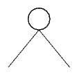
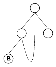
A natural deduction proof is usually presented in a tree-like notation
where the derived formula is the root, usually written at the bottom.
The leaves of the tree are formulae referred to as assumptions.
The inner nodes of the tree correspond to applications of the
derivation rules detailed further below.
Each rule is written as a horizontal
line with exactly one formula (the conclusion) below that line
and one or more formulae (the premises) above that line. In
addition to this, some rules are written with one or more formulae in
square brackets to the right of the line. These are assumptions that
this rule discharges. In order to be a valid derivation for a tautology,
all of the assumptions found in leaves of the tree must be
discharged (noted by being put in square brackets).
An assumption is discharged if one of
its ancestors in the tree is a rule that discharges it. The
following is an example of a valid derivation:
[(A→⊥)→⊥] [A→⊥]
⊥
[A→⊥]
A
[(A→⊥)→⊥]
((A→⊥)→⊥)→A
1.2.3 Rules of Inference
To get a complete (and correct) calculus for classical propositional
logic, the following three rules (more properly rule
schemata) of inference are sufficient. All other
rules can be derived using just these three.
X1
[X0]
X0→X1
→ introduction
X0 X0→X1
X1
→ elimination/modus ponens
⊥
[X0→⊥]
X0
reductio ad absurdum/tertium non datur
2 The Domino Metaphor
2.1 Introduction
Dominoes is a game played with rectangular tiles. Each tile is divided
in two squares that are labelled with number symbols like the faces of a
standard dice. There are many games that can be played with domino tiles.
One of the most simple variants of the Dominoes game begins with a single
tile and each player having a pile of tiles. A player may play one of
his tiles by connecting it to an unconnected end of a tile played
earlier. The two connected squares must have matching numbers.
Natural deduction follows similar principles. It is very common to begin
with the tautology to prove and to apply inference rules backwards until
only discharged assumptions remain. When seen as a domino game, each
inference rule corresponds to a domino tile, with premise and
conclusion corresponding to the labels on the two squares of the tile.
The main differences to a real game of dominoes are
- Inference rules are directed. A premise can only be connected to
a conclusion and vice versa.
- The modus ponens inference rule has two premises and
consequently three connection points.
Aside from these differences the domino game models natural deduction
rather well. The number of different square labels needs to be higher than
used for a real domino game, of course. Although arbitrary symbols
could be chosen, it is desirable to have a systematic mapping from
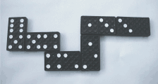
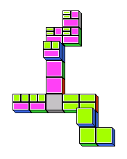
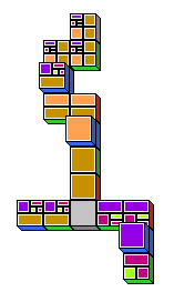
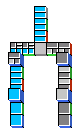
formulae to square labels. The picture below demonstrates a possible
rendering of a proof for ⊥→(A→(B→(C→D))) as a game of dominoes.
The proof does not use modus ponens, so there are no branches.
Note that discharged assumptions are not shown in the picture.
2.2 Mapping Derivations to Dominoes
The following paragraphs give a detailed description of the mapping
between natural deduction derivations and the dominoes game as it has
been implemented. As mentioned before, the domino system
described here is not a new logical formalism. It is simply a different
notation for natural deduction, used to create a special kind of Graphical
User Interface (GUI) for an interactive theorem prover.
Consequently, the mapping described here
is a straightforward 1-to-1 mapping, so that the
correctness and completeness results for natural deduction apply
unchanged.
2.2.1 Mapping Formulae to Color Patterns
The labels used on the domino tiles correspond to the premises and
conclusions of the inference rules. While it would be possible to use a
formula directly in its textual form to label a square of a tile, this
is not desirable in practice. The space available on a domino tile is
very limited, so the formula would have to be printed in a very small
font when presenting the tile on screen. Furthermore, as the domino
notation is intended only for use in a GUI, it is only reasonable to
make full use of the graphical nature of the environment by presenting
formulae in a way that offers better visual clues than traditional
text notations. Last but not least, a colorful presentation makes
the program overall more enjoyable.
For the purpose of the following definition, let pattern(X0) denote
the rectangular pattern assigned to the formula X0. pattern(X0)
is defined as follows:
- Case X0=⊥ :
-
The pattern for ⊥ is a solid red rectangle framed by
a black and a white border:

- Case X0=A, X0=B, ... :
-
Every propositional variable is assigned a unique color that is
not white, black or red. The pattern for a propositional variable
is a solid rectangle of the variable's assigned color,
framed by a black and a white border.
Examples: pattern(A) =  , pattern(B) =
- Case X0=(X1→X2) :
-
The pattern for an implication is a rectangle R that is split in
two rectangles R1 and R2.
The pattern of R1 is pattern(X1) and the pattern of R2 is
pattern(X2). The split is done according to the following rules:
- If R is not the result of a split, i.e. if X0 is not part
of another implication, the split is a horizontal split, with R1
as the top and R2 as the bottom rectangle.
- If R is the result of a split, i.e. if X0 is an operand of
an implication for which the pattern is being computed, the
split axis for R is perpendicular to that of its parent rectangle.
If R is split horizontally, then R1 is the top rectangle and
R2 is the bottom rectangle. If R is split vertically, R1 is the
left and R2 is the right rectangle.
Examples:
pattern(A→B) = ,
pattern((A→B)→C) =
,
pattern((A→B)→C) = ,
pattern(A→(B→C)) =
,
pattern(A→(B→C)) = ,
pattern(((A→B)→C)→D) =
,
pattern(((A→B)→C)→D) = ,
pattern((A→B)→(C→D)) =
,
pattern((A→B)→(C→D)) =
It is obvious that with the alternating split axis and the rule
that the first split must be horizontal, it is always possible to
unambiguously determine the exact sequence of splits that lead to any
given pattern.
The black and white borders around the rectangles make sure
that two adjacent rectangles can never appear as a single,
larger rectangle, even if they have the same color.
As a consequence, the mapping from formula to pattern is easily
reversed.
2.2.2 Mapping Inference Rules to Tiles
Now that each formula has been assigned a color pattern, mapping
inference rules to domino tiles is trivial. A rule is characterised
by its premises, its conclusion and the assumptions it discharges.
All of these are formulae. Each formula X0 is represented by a block
that has pattern(X0) on its top.
All of these blocks are
connected to form the tile that represents the inference rule.
One important thing has to be taken into account. Conclusion, premises
and
discharged assumptions play different roles and therefore need to be
distinguished. The representation presented here distinguishes them
by the color of the sides of the blocks. The conclusion of a derivation
rule is represented by a block with red sides, the premises are
represented by blocks with green sides and the discharged assumptions
are represented by blocks with blue sides. These blocks will be
referred to as red blocks, green blocks and blue blocks
respectively.
The arrangement of the blocks is not important as long as the blocks
that represent conclusion and premises are not completely surrounded
by other
blocks, which would make the connection of another tile impossible.
Because keeping track of
the discharged assumptions is very important, the respective blocks are
presented as being stacked on top of another block, which makes them
stick out visually. The following pictures show examples of
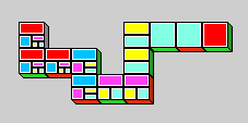
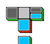
instances of the three inference rules of natural deduction:
A
[B]
B→A
is represented as 
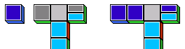
A→B (A→B)→C
C
is represented as 
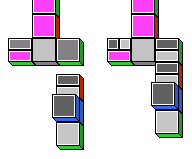
⊥
[C→⊥]
C
is represented as 
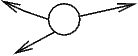
2.2.3 The Rules of the Game
The rules of the game are easy. The game begins with a single tile
that has a single green block that represents the tautology to be
proven and no red block. This would correspond to a derivation rule
with just a premise and no conclusion. Every turn, a
tile representing a derivation rule is connected to a tile placed
earlier. The red block of the newly placed tile must be connected
to exactly one green block of the other tile. Two green blocks can not
be connected. The usual domino rule applies that the two blocks being
connected must show the same pattern.
In a real domino game, players only have a limited number
of tiles. In natural deduction domino, all tiles corresponding to
instances of the three derivation rules are available without
limitations at all times.
The structure built up during the course of the game is
a tree with the start tile as root and one or more green blocks as
leaves. This tree will be referred to as the domino tree.
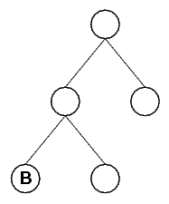
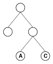
A leaf of the domino tree is said to be closed
if the green block that
marks this leaf shows the same pattern as at least one blue block
of the tile the leaf belongs to or a tile that is an ancestor of this
tile in the domino tree. If all leaves are closed, the domino tree is
said to be closed. Otherwise it is open.
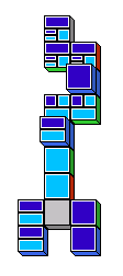
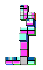
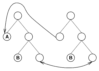
The following pictures show some closed and some
open domino trees. To emphasize closed leaves, blue blocks
have been connected to them. This is just a matter of presentation and
not an actual part of the mapping between proof and domino game.
The game is finished when all leaves of the domino tree are
closed. Rules for scoring and determining which player has won
the game are not provided here because they are not relevant for the
logical mapping between domino game and natural deduction.
It is easy to see that any closed domino tree for a game finished
according to
the above rules corresponds to a valid derivation of a tautology.
Likewise, every correct derivation can be transformed into a domino
tree.
Domino trees are just a different notation for natural deduction
derivations.
3 The Domino Program
3.1 Program Description
The domino metaphor for natural deduction has been implemented in
Java.
The program is available at [5]. It can be downloaded
for local use or played on-line with Java-enabled browsers. Full
source code is included.
The program has one main window that displays the domino tree for
the current game. Domino
tiles are shown in an isometric perspective. The blocks are labelled with
color patterns as have been described, with a small extension.
Because the number of visually distinct colors is limited, multi-letter
propositional variables are not represented by a single-color solid
rectangle. Instead they are represented by concentric rectangles, each
of which represents a single-letter. This extended
mapping is still unique and reversible.
The program is controlled by the mouse or alternatively by a combination
of mouse and keyboard. The user requests new domino tiles and places
them in the main window according to the rules that have been explained.
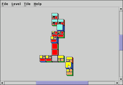
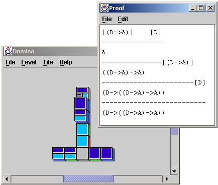
The program offers some useful features beyond the actual domino game.
The perhaps most important feature is the ability to create a text
representation in standard notation of the proof corresponding to the
current domino tree. This allows a direct comparison between the two
notations.
Another interesting feature is the ability to create custom tiles as
shortcuts for combinations of several tiles. Saving and loading these
custom tiles is supported. The format used for the tile files is an
easy to read and edit text format which allows the creation of tiles
that go beyond classical logic and the rules described in this paper.
It would be possible to restrict the game to intuitionistic logic,
for example.
The program implements the mapping between natural deduction and dominoes
with some differences compared to the description given in this
paper. The first difference is the
terminology used in the manual and the menus.
Terms such as "modus ponens" and "tautology" are avoided. Instead
non-technical names are used that are more appropriate for a computer
game. The intention is to increase the appeal of the program to people
without a scientific background. This is desirable because one of the
goals of this project has been to create an environment that even
persons without any background in logic should be able to use.
Although no further research in this direction has been done as part
of this project, studying the way the domino program is used by
people without background knowledge could yield interesting results.
Another difference is that by default the start tile presented by the
program does not correspond to the rules of the game as they have
been presented in this article. Because it is so common to begin
the proof by applying
the → introduction rule to the tautology to be proven in order to
simplify it and discharge assumptions at the same time, the game
automatically applies the → introduction rule as often as is possible,
thereby simplifying the pattern on the start tile's green block while at
the same time providing some blue blocks. This does not affect
correctness or completeness and the feature can be turned off in the
Level menu.
The most important difference between the domino metaphor as discussed
in this paper and the actual implementation concerns the
tiles corresponding to inference rules. To play the game, all tiles
corresponding to instances of the derivation rules must be available
to a player. However, there is an infinite number of such instances,
which means that it is unfeasible to provide the tiles explicitly. One
possible way to solve this problem would be to have the user specify the
premises and conclusions a rule is to be instantiated with. This would
either require the entering of formulae which would undermine the whole
concept of using a purely visual representation, or it would require
some way to specify the patterns directly, which would likely be
as inconvenient.
The solution implemented in the Domino program is different. It could be
described as indirect or lazy instantiation. It is based on the
observation that an inference rule does not need to be instantiated
right away. This is best explained with an example. Let's assume
the user wants to derive A→(B→A) (i.e. the corresponding tile is the
start tile). As a first step he wants to attach a
tile that corresponds to the following inference rule:
B→A
[A]
A→(B→A)
This rule is an instance of the → introduction rule (schema):
X1
[X0]
X0→X1
When the user requests an → introduction tile, a dialog box could be
presented, asking him to enter formulae for X0 and X1 and the
user would enter A and B→A respectively. The tile would be created
and the user could attach it to the A→(B→A) block of the start
tile. However, it turns out that requiring the user to enter bindings
for X0 and X1 directly is unnecessary.
The domino rules say that two tiles can
only be connected if the adjacent squares show the same pattern. If the
user wants to attach an → introduction tile to an A→(B→A) block,
there is no choice for X0 and X1. If they are not A and A→B
respectively, the tiles cannot be connected. To take advantage of
this observation, when the
user requests an → introduction tile, a meta-tile is created
that corresponds to the schema without being an instance.
For the purpose of constructing the patterns for the
blocks of this tile the unbound variables X0 and X1 in the schema
formulae are treated as if they were bound variables distinct from
all other bound variables.
The following is an example of such a meta-tile:

Here, shades of gray are used in the patterns as colors for the unbound
variables. This doesn't create a conflict because the program does not
use shades of gray for bound propositional variables.
When this meta-tile is
connected to another tile, the gray rectangles are replaced with the
corresponding patterns on the block the tile is connected to.
In other words, the
tile is instantiated indirectly through the connection made.
This indirect instantiation has an interesting effect when modus
ponens tiles are used. As you can see in the following picture,
attaching a modus ponens tile to another tile does not bind all of
its wildcard patterns.
This is easy to understand when you look at the modus ponens
inference rule:
X0 X0→X1
X1
The variable X0 is not present in the conclusion so when the red
block that corresponds to the conclusion is connected to a green block,
the variable X0 does not matter at all. To bind this variable, too,
another tile is required. In the following picture, a blue block is
attached to close a leaf. This binds X0.
It is possible to connect other meta-tiles to the branches of a modus
ponens
tile, as demonstrated in the following picture. This does not bind the
wildcard patterns, but it merges the structural information they
provide. In this case one wildcard pattern has a split and the other
has not. The split pattern is more specific than the unsplit pattern,
because the corresponding formula must have at least one →, whereas
the unsplit pattern can represent any formula whatsoever.
The domino rule mandates that both blocks must show the same pattern.
The information contained in the split pattern that it stands for an
implication must not be lost obviously, so the unsplit pattern changes
to match the split pattern.
It is important to understand that the introduction of meta-tiles does
not in any way extend or change the underlying logic. Each wildcard
pattern on a meta-tile is just a placeholder for a pattern representing a
formula that contains no unbound variables. This applies even if a
finished domino tree still contains wildcard patterns like the following:
Because the inference rule schemata make no restrictions regarding
instantiation of unbound variables,
the proof corresponding to the above tree is valid,
regardless of the formulae bound to the remaining unbound variables.
So, in order to eliminate the remaining unbound propositional variables,
it is permissible to replace them all with the bound variable A,
for instance.
3.2 Implementation Overview
The following sections will take a look at some aspects of
the program's implementation that concern the internal
representation of formulae and domino trees. For a comprehensive and
in-depth look at the implementation, readers are referred to the
source code that is provided with the program and the javadoc
documentation that can be generated from it.
The source code is split across three packages: domino.core,
domino.ui and domino.logic. The classes that will be
discussed here all belong to the domino.logic package.
This package can be divided into three layers. The first layer is
the formula layer, provided by the FormulaSyntaxNet
class that
is used for the low-level representation of formulae. Building on top
of and very closely connected to this layer is the
domino tree layer,
provided by the FormulaDominoTree class. Above this layer is
the application layer formed by the classes/programs that make
use of FormulaDominoTrees as representations of natural
deduction derivations.
3.3 The FormulaSyntaxNet Class
One question that stood at the beginning of the development of the
domino program was that of how domino trees should be represented
internally. This question inevitably lead to the question of how formulae
should be stored and manipulated.
Although mathematically harmless, the desire to implement the indirect
instantiation feature in the program's user interface turned out
to be the dominating factor when designing the data structures dealing
with formulae. Most of the complexity but also the flexibility of the
FormulaSyntaxNet and FormulaDominoTree classes is
a direct consequence of design choices made to add support for this
feature.
In order to support indirect instantiation, it has to be possible to
unify two or more formulae. Unification identifies the unbound
propositional variables in one formula with parts of another formula
and vice versa, with the goal of making the two formulae equivalent.
If the formula A→(B→C) is unified with the formula X0→X1 for
instance, X0 is bound to A and X1 is bound to (B→C). With
this binding, the second formula is equivalent to the first. A
slightly more complicated example is the unification of X0→(B→C) with
A→X1 that results in the same bindings for X0 and X1.
Not all formulae can be unified. The unification of A→B and X0→C
is not possible because B and C are different bound propositional
variables that can not be identified with each other. The unification
of A→(X0→X1) with A→B is also not possible, because no binding
of X0 and X1 can make X0→X1 equivalent to B.
Looking at the simple examples above, unification seems to be easy to
implement using a table that maps unbound variables to the formulae they
are bound to. Unfortunately, things are not as easy as the simple
examples suggest. One issue that has to be dealt with is the possibility
that a unification occurs between two unbound variables as happens when
unifying X0→X1 with X2→X3. This unification leaves all four
variables unbound. It does, however, establish a connection between
X0 and X2 and a connection between X1 and X3. Suppose that,
after this unification, another unification takes place, unifying
X0→X1 with A→B, this unification must bind not only X0 and X1,
but also X2 and X3. A series of unifications of formulae containing
many unbound propositional variables can quickly lead to a complex
web of connections.
Even with the complications arising from unifying unbound variables with
each other, a simple table-based approach seems possible. Unbound
variables that have been unified could be made to point to a common entry
in the table and successive unifications would update the respective
entries and pointers. This method is simple to implement and works well
if unifications are final. Applied to the domino metaphor, unifications
being final corresponds to a rule that says that a domino tile can
not be removed
once it has been placed. Indeed, such a rule exists in real domino games,
but with such a rule it would be possible for the user to find himself
in a dead end during the game.
So it is essential to
give the user the ability to remove tiles from a domino tree.
Unfortunately, providing this feature makes the implementation more
difficult. An easy way to implement the feature would be to store
a history of unifications, similar to the undo information in a text
editor. This approach would limit the user to removing tiles in the
order they were placed. But users will often
want to remove tiles from different leaves of the domino tree and would
perceive the restrictions imposed on their ability to do so as arbitrary
and counter-intuitive.
To address all of the issues mentioned above, the data structure for
managing formulae and unifications needs to be more complex than a
simple table that maps unbound variables to their bindings. The data
structure that was chosen for the domino program and implemented in
the FormulaSyntaxNet class is a net of interconnected trees.
The following paragraphs will take a look at this structure.
As long as no unifications are involved, a FormulaSyntaxNet
is just a kind of syntax tree. This tree can have three types of node.
The first category is made up by bound leaf nodes. A bound leaf
is a leaf that is labelled with the name of a bound propositional
variable as depicted in the following picture:

The second node type is the unbound leaf node. An unbound
leaf is a leaf node that does not have a label.

The third category of nodes are the branch nodes. In a syntax
tree a branch node corresponds to an operator, that has its operands
as branches. Because → is the only operator that can occur
in the formulae used
here, all branch nodes are binary nodes whose left branch is the
premise of an implication and whose right branch is the conclusion.
With branch nodes, unbound and bound leaves, all the formulae needed for
classical propositional logic can be represented. The following
pictures show the FormulaSyntaxNets for
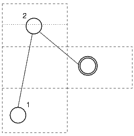
(B→X0)→X1, X2→(A→C) and (A→X3)→X4 respectively.
Notice that the variable names used for
unbound variables in the formulae are arbitrary as long as the same
unbound variable has the same name whenever it occurs and two different
unbound variables have different names. In the tree structure, names
are not necessary for unbound nodes. If the same unbound variable occurs
multiple times in a formula, the corresponding FormulaSyntaxNet
contains only one unbound node for that variable. This can lead to
deformed trees where multiple different branches have the same leaf.
When dealing with FormulaSyntaxNets, you should keep in mind
that while every formula has a corresponding FormulaSyntaxNet,
not every FormulaSyntaxNet corresponds to a formula. A
FormulaSyntaxNet can be recursive as is demonstrated in the
following picture. This FormulaSyntaxNet would correspond to
an infinite formula, but such formulae are not permitted here.
Now that the representation of basic formulae as FormulaSyntaxNets
has been described, unification will be introduced. For this purpose,
a fourth node type, the forward node, is necessary. Forward
nodes are an extension of unbound leaves. A forward node carries
a reference to every node that is equivalent to it because of
unifications. So, an unbound leaf is a forward node that has not been
unified with any other node. Notice, that a forward node may refer to
other forward nodes and these refer back to it, because equivalence
is symmetrical.
The name forward node refers to the way
most algorithms working on FormulaSyntaxNets treat them. A
forward node that has at least one reference (i.e. a forward node that
is not an unbound leaf) is processed by picking one of the nodes it
refers to and processing that node. In other words, the processing is
forwarded to one of the referenced nodes. Because all nodes referred
to by a forward node are equivalent, it does not matter which one
is picked for processing. This is only a simplified
description, of course. In practice it is at least necessary to take
precautions to prevent endless loops, because the node being picked could
itself be a forward node, and as such would have a reference back to
the original forward node which must not be picked again.
Forward nodes are only created when unifying
FormulaSyntaxNets. The following
pseudo-code gives an overview of the unification algorithm. In this
pseudo-code, as well as the actual Java implementation, a variable of
type FormulaSyntaxNet refers to a single node within the net.
unify(FormulaSyntaxNet a, FormulaSyntaxNet b)
{
  if (a is the same node as b OR
      a and b have already been unified) return

  if (a is bound leaf AND b is bound leaf)
  {
    if (label of a != label of b)
        throw UnificationNotPossibleException
  }
  else
  if (a is branch node AND b is branch node)
  {
    unify(left branch of a, left branch of b)
    unify(right branch of a, right branch of b)
  }
  else
  if (a is unbound or forward node OR b is unbound or forward node)
  {
    let x be the first unbound or forward node in the list (a,b)
    let y be the other node

    if (y is bound node or branch)
    {
      add a reference to y to x's list of references

      for every node p from x's list of references
      {
        unify(p,y)
      }
    }
    else if (y is unbound or forward node)
    {
      add a reference to y to x's list of references
      add a reference to x to y's list of references

      for every pair of nodes (p,q)
      where p is from x's list of references
      and   q is from y's list if references
      {
        unify(p,q)
      }
    }
  }
  else throw UnificationNotPossibleException
}
The following picture shows the result of unifying the formula
A→(B→X0) with the formula X1→(B→X2).
There are some things that the above algorithm does not show but that
are important nevertheless. One thing that is missing above is code to
remove all newly created references if the unification fails, to
restore the nets a and b to their original states.
Another omission is code to recognize unifications that would cause
the creation of a recursive FormulaSyntaxNet. As has been
mentioned, a recursive FormulaSyntaxNet corresponds to an
infinite formula which is not allowed. Readers interested
in how these details are handled in the Domino program should consult
the source code.
3.4 The FormulaDominoTree Class
The FormulaSyntaxNet class provides the functionality needed
to work with formulae connected through unifications no matter how
complex. A FormulaSyntaxNet can even represent an infinite
formula. It is obvious that for implementing the domino metaphor
all this flexibility is mostly unnecessary. Furthermore,
FormulaSyntaxNets with all their pointers and their complex
interconnections are difficult to work with and a real nightmare to
debug.
To address these issues, the FormulaDominoTree class has been
introduced as a layer above FormulaSyntaxNet.
FormulaDominoTrees provide a higher level of abstraction
because they work on the level of domino tiles and domino trees. This
serves two purposes. First, it reduces the amount of
application layer code, because
one operation on a FormulaDominoTree may perform many operations
on the underlying FormulaSyntaxNet(s). The second and more
important purpose is to enforce the
rules of natural deduction. The FormulaDominoTree class is
the implementation of the domino tree as it was introduced earlier,
and as such directly corresponds to natural deduction. It is
possible to automatically convert any FormulaDominoTree to
the standard textual notation for derivations. The
ProofFormatter class implements this conversion.
A single instance of the FormulaDominoTree class represents
a derivation rule. It has one FormulaSyntaxNet that represents
the conclusion, one for each premise and one for each discharged
assumption. These FormulaSyntaxNets are not separate. Whenever
possible they physically share nodes, so that within an atomic
FormulaDominoTree instance, unifications are not necessary.
Consequentially, an isolated FormulaDominoTree does
not have any forward nodes in its FormulaSyntaxNets.
In addition to the FormulaSyntaxNets, a
FormulaDominoTree holds references to other
FormulaDominoTrees. There is one reference for the conclusion and
one for each premise. These references are used to connect
atomic FormulaDominoTree instances to form a tree, just like
domino tiles are connected to form the domino tree. Whenever the
conclusion connection of one FormulaDominoTree is connected to
a matching premise connection of another FormulaDominoTree,
the respective references are updated and the corresponding
FormulaSyntaxNets are unified. This directly corresponds to the
connecting of domino tiles in the domino program to build the
domino tree. Notice that, although
technically FormulaDominoTree is the class of a single node of
the tree, the name will also be used to refer to the tree that is rooted
at that node.
The domino game uses three types of atomic
FormulaDominoTrees that correspond to the three types of
domino tiles in the domino metaphor, which in turn correspond to the
three inference rules presented for classical propositional logic.
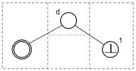
The following pictures illustrate these three types. In the pictures,
the node that corresponds to the conclusion of the rule has a double
border, numbers mark the unbound leaf nodes corresponding to the premises
and the letter "d" marks the FormulaSyntaxNet representing
a discharged assumption.
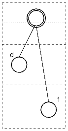
There is a fourth
type of FormulaDominoTree that is used to close a leaf of
the domino tree just like the blue blocks are used in the domino program.
This special FormulaDominoTree has only one
FormulaSyntaxNet that is unified with a discharged assumption of
an ancestor FormulaDominoTree. With these four atomic
FormulaDominoTrees, any domino tree can be represented.
The
following sequence of pictures shows how the FormulaDominoTree
is built up during the first steps of a proof for
the formula A→((A→B)→B),
using the diagram notation described above.

When the FormulaSyntaxNet class was introduced, the problem
of removing tiles from a domino tree was already mentioned.
With the FormulaDominoTree class this problem is now easy to
solve.
Whenever a subtree of a FormulaDominoTree is removed, all
that has to be done is to undo unifications with
FormulaSyntaxNets belonging to the subtree being removed.
The algorithm implemented to do this is very simple. It removes
all forward node connections from all FormulaSyntaxNets
and after removing the subtree reunifies those corresponding to
premise/conclusion connections that remain. This algorithm works
because atomic FormulaDominoTrees never
contain forward nodes since their FormulaSyntaxNets
physically share nodes. All forward node connections
in all FormulaSyntaxNets within a FormulaDominoTree are the
result of connecting atomic FormulaDominoTrees, and as a
consequence they can all be reconstructed from the premise/conclusion
connections.
The above solution is obviously not very efficient. In some special
cases, the program uses a more efficient algorithm that works by
assigning
every FormulaSyntaxNet a reference to the
FormulaDominoTree that contains it. Using these owner
references it is easy to limit the removal of connections to those
FormulaSyntaxNet nodes that belong to the domino tile being
removed. However, one issue makes this method unfit for general
use. The problem is illustrated in the following picture sequence
(for clarity's sake only three FormulaSyntaxNet nodes are shown
instead of three complete FormulaDominoTrees).
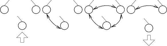
The illustration demonstrates that when an unbound leaf X0 is unified
with another unbound leaf X1 and then with yet another unbound leaf
X2, this creates a
cross-connection between X1 and X2. This happens because forward
nodes by definition have references to all nodes that are equivalent
(through unification), and equivalence is transitive.
The cross-connection remains even after removing X0, because it is a
connection between nodes that belong to different
FormulaDominoTrees than X0, so that the owner-based algorithm
does not touch it. While the domino tree
remains logically valid, this effect is confusing for the user and
might in some cases even result in a tree that can not be closed
anymore. This issue can only arise when the same discharged assumption
is used to close two different leaves. To eliminate the problem,
the cross-unifications in question would have to be tracked, but
this is currently not implemented because the trees as
they occur when using the program are so small that the performance
loss of the complete rebuilding algorithm has no practical
significance.
3.5 FormulaDominoTree Applications
During the development of the main program, a few other interesting
programs were written that make use of the FormulaDominoTree class.
They are all similar in the respect that they construct
FormulaDominoTrees
by repeatedly connecting copies of the three
basic FormulaDominoTrees
that correspond to the three rules of inference. In addition to this,
discharged assumption FormulaDominoTrees are used to close leaves.
This process is repeated until
a tree has been generated with no open leaves remaining.
This tree is converted to
an ASCII representation of the corresponding proof in standard notation
using the ProofFormatter class and then written
to standard output.
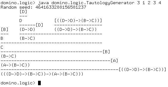
3.5.1 TautologyGenerator
This class provides a method for generating a propositional logic
tautology with a proof in the form of a FormulaDominoTree.
When used as a stand-alone program, the tautology is output as an infix
formula together with a proof in standard notation. Parameters can
be passed to influence the relative frequency with which the
different inference rules are used in the proof. Note, that the
proof is by no means a minimal proof. The program will often
generate complex proofs for trivial tautologies.
The domino.core.LevelGenerator is a slightly modified
version of this class that aims to produce more complex tautologies
to be used as levels in the domino game.
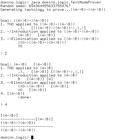
3.5.2 TextModeProver
In a way this class can be seen as the ancestor of the domino program.
It offers a simple text mode interface for proving a tautology.
The program begins with the tautology to prove and enumerates all
possibilities for applying an inference rule, presenting the new
premises that have to be proven if a rule is applied and the
assumptions the rule discharges. The user simply enters a number
to select one of the presented possibilities and the respective
rule is applied. This continues until the FormulaDominoTree
that is built up in this manner is closed. Finally the constructed
proof is output in standard notation.
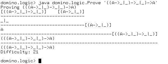
3.5.3 Prove
This is a particularly interesting class. It works as a stand-alone
program that takes a tautology as
input and finds a proof for it. The program does this by
constructing FormulaDominoTrees beginning with the tautology
to be proven, until a closed FormulaDominoTree has been found.
Because breadth-first search consumes too much time and resources, the
program uses heuristics to keep the number of trees low and to focus
on those trees that are more likely to lead to a fast conclusion of the
search. Because of these heuristics, the constructed proof is not
minimal, but this is compensated by a proof-simplification step that
is usually capable of reducing the proof to a minimal one.
No attempt was made to ensure that the heuristics employed
maintain the completeness of the breadth-first search, i.e. it is
well possible that a tautology exists for which the program can not
find a proof because the heuristics discard all trees that would prove
it. However, with the several hundred tautologies tested with this
program this problem has not been observed.
It needs to be said that Prove was not written to be a good
implementation of an automatic theorem prover. Prove's
usefulness
lies in the fact that it can rate the difficulty of a proof with
respect to the domino metaphor. It assigns difficulty points to each
application of an inference rule in the proof it finds, based on
heuristics determined
while playing with the domino program. This rating was used to
sort the levels included in the game by ascending difficulty.
4 Conclusion
Although the domino game in its present state is limited to
propositional logic, it permits
some interesting observations regarding the general feasibility and
effectiveness of using a purely graphical system for constructing proofs.
One evident advantage is the compactness
of presentation that a graphical system can offer. When you compare a
domino tree with its corresponding proof in traditional notation, the
domino tree is usually much smaller. In addition to this, the patterns
and colors used by the domino game give much better visual clues than
the corresponding textual formulae, especially when they are long and
complex.
Another advantage has already been hinted at in the introduction by
Peirce's statement that "all knowledge without exception
comes from observation". An abstract graphical system offers a lot of
room for playing around and observing patterns, something that is
difficult with traditional textual systems because they are burdened
with semantics that lead the mind into a certain direction.
Finally, a positive aspect that must not be overlooked is the fact that
the domino game offers a more interesting experience than textual
interfaces. This can improve a user's motivation and endurance when
working on a difficult problem.
A purely graphical proving system does not only have advantages.
One serious disadvantage of purely graphical reasoning systems
is the fact that much of the background
knowledge a user may have about logic does not translate easily to
the graphical system. A lot of things have to be relearned. One example
concerning the domino metaphor is the recognition of trivial truths such
as A→A. The ability to spot these trivial tautologies in textual
notation does not automatically result in the ability to spot the
corresponding color patterns when working with the domino game.
Another disadvantage is that an abstract graphical system is a step
further away from the problem domain. Results achieved through
manipulations in the abstract system do not usually have a straightforward
reading with regards to the problem being solved. A translation step is
required. The same is true in the other direction. Facts about the
problem domain can not be used without being first translated into an
abstract presentation. As a consequence it is difficult to make use of
semantic background information that does not fit into the formal
framework.
Despite the disadvantages, the results show that the usefulness of
graphical concepts is not limited
to teaching tools, but that it can actually improve the effectiveness
of an interactive reasoning system's user interface.
More research in this area is
certainly required, especially concerning ways to combine the traditional
formula-based approach with diagrammatic reasoning to get the best of
both worlds.
But graphical reasoning systems are not only interesting tools for
logicians. They could be used to explore aspects of the human brain
regarding logical thinking.
It could be interesting to examine the way the domino program is used by
different people, both with and without background knowledge about logic.
PET scans could be used to determine if using the domino program
causes activity in the same areas of the brain as reasoning
with the conventional formula-based notation,
or if the same result (a proof of a
tautology) is achieved in a different way.
Because the game does not require the ability to read or write or in fact
any language skills whatsoever, it could also provide
a suitable platform for studies involving children, illiterate people or
persons with mental disabilities.
Studies using the domino game could provide
new insights about how logical thinking works in the brain, especially
in the absence of language.
References
[1]
C.S. Peirce, J.F. Sowa, Existential Graphs,
http://www.jfsowa.com/peirce/ms514.htm
[2]
J. Howse, F. Molina, J. Taylor, SD2: A Sound and Complete Diagrammatic Reasoning System,
Proceedings VL 2000: IEEE Symposium on Visual Languages,
Seattle, IEEE Computer Society Press 2000, p. 127-136
,
http://citeseer.nj.nec.com/512087.html
[3]
J. Barwise, J. Etchemendy, Hyperproof,
CSLI Publications, Cambridge University Press
,
http://www-csli.stanford.edu/hp/Logic-software.html
[4]
G. Gentzen, Untersuchungen über das logische Schließen I-II,
Mathematische Zeitschrift, vol. 39 (1935), p. 176-210, 405-431
,
http://gdz-srv2.sub.uni-goettingen.de/agora_docs/17147TABLE_OF_CONTENTS.html
[5]
M.S. Benkmann, Natural Deduction Domino Java Applet,
http://www.winterdrache.de/freeware/domino/index.html